Natural Language Processing

Natural Language processing is a branch of artificial intelligence deals with interaction between machines and humans using Natural Language.

NLP is difficult because, first the words must be understood and then they must be combined together to undertanding the underlying meaning, emotion behind it.

Syntactic analysis and Symantic analysis are the techniques used to complete NLP tasks and these techniques rely on machine learning to derive meaning from human language.

Syntactic analysis uses the grammatical rules on the sentence to make sense of it or to get valuable information from it and Symantic analysis uses words and how they are interpreted.

We can levearge Machine Learning to implement the techniques of Natual Language problem.

Embeddings

Machine Learning models like numbers and they hate anythinh other than numbers they really do. To get useful information via machine learning, first step is to convert text data into numbers. This post discusses about few methods,

One-Hot Encoding

Encoding text to numbers. Create a zero vector to the length of the vocabulary(number of unique words on the data) and assign 1 at the index o the word. By doing this what we achieve is called a sparse vector, meaning most indices of the vector are zeros. To form a sentence, concatenate one-hot encoding of the words.

Let’s consider a vocabulary with 15,000 words and we encode all of them, what we get is 99.99% of zeros in our data which is really inefficient for training.

Integer Encoding with unique numbers

Let’s switch to use an unique number for each words in the vocabulary. This is efficient thean the above because we’ll get a dense vector instead of sparse vector.

But in this method, we lose valuable information to amke something out of the data. Realationship between words is lost. Integer encoding can be challenging for models to interpret, because there is no relationship between similar words and the encodings are alos differnet. This leads to feature-weight combination which is not meaningful.

This where embedding comes in

Word Embeddings

Word embedding is an efficient dense vector way where similar words have similar encodings. Embeddings are floating point vectors, whose values doesn’t need to be setup manually. The advantage is the embedding values are learned during training similar to weights of a dense layer. The length of the vector is a parameter to be specified.

The embedding length ranges from 8-dimensional for small datasets to 1024-dimensions for large datasets but requires more data to learn.

Checkout this notebook for detailed walk through of word embeddings in TensorFlow

Visulaization of word embeddings on tensorflow embedding projector

Limitations of Feed Forward Networks

Feed forward network or perceptron, given an input produces an output. Here both input and output are static or of fixed shape. Let’s consider a text sequence I am learning Deep Learning. All the words are splitted and fed into the neural network and we gt a output but we lose the information between the sequence since each word is treated as a seperate entity.

To process sequence data, we need the information from past memory (i.e) while processing am we need the context of learning.. This is not possible in traditional feed forward network. Toa achieve this we need recurrence, meaning both current input and previous state is required. Recurrent Neural Network does exactly this, it maintains an internal state of the previous timesteps by an internal for loop.

Recurrent Neural Networks

Recurrent Neural Network are powerful for modelling sequence data such as time series and natural language.

The basic defintion of RNN is RNN's have a internal `for loop` to iterate over timestamps of sequence data. The RNN's have an internal state that encodes information about the timestamps it has seen.

Let’s dive deeper,

So we have established RNN’s has a sense of recurrence, how is this done?

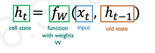
RNN’s have a hidden state updated at each timestep while a sequence is getting processed, where **h_{t** is the hidden state.}

To calculate **h_{t** at every time step, recurrence relation is applied at every time step as below,}

One important point is the same function and parameters(weights) are used at every timestep of processing the sequence. But these weights will be learned and updated during trianing.

RNN intution in Pseudo Code

In this pseudo code, we’re trying to predict tthe next word in sequence

my_rnn = RNN()
hidden_state = [0,0,0,0]

sentence = ["I", "am", "learning", ""RNN]

for word in sentence:
    prediction, hidden_state = my_rnn(word, hidden_state)

next_word_prediction = prediction

RNN State Update and Output

When an input vector The hidden state is updated as below.

In hidden state caluclation there are two elements, dot product of hidden state weigh matrix and hidden state encoded of all the previous time stamp is summed with weight matrix and current input dot product. The sum is passed to tanh activation.

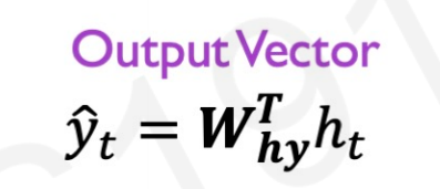
From the hidden state the output y is equal to product of weight matrix and hidden state.

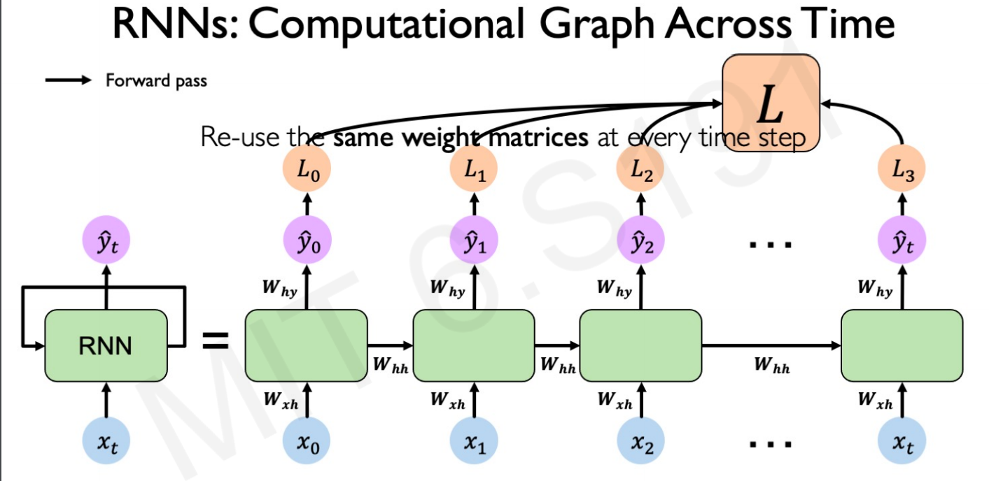
RNN’s computational graph across time

When a sequence is getting processed in an RNN, we’ll get a output and hidden state at each time step. Similary we’ll get a loss for every time step, a main loss os derived from these. This is main loss which the model will try to minimize during trainig.

But the weights will remain the same for entire sequence.

Sequence Modeling: Design Criteria

To model sequences, we need:

Handle variable-length sequences
Track long-term dependencies
Maintain information about order
Share parameters across the sequence

RNN’s meet all these design criteria.

Backpropogation Through Time

This is the actual algorithm used to train RNN.

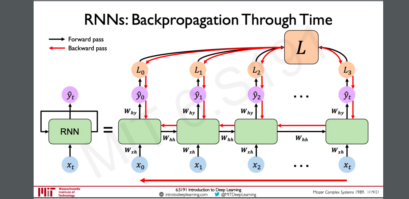
Unlinke in a feed forward network where the backpropogation takes at a single timestep. In RNN there are loss at each timestep for a sequence.

In RNN’s backpropogation is stated at overall loss through each individual loss and then backpropgated across each timestep in the sequence, this is why it’s called as BPPT.

Gradient issues

To compute gradient of initial hidden state invloves many factoes of weight matrices and repeated gradient computation.

Many weight values greater than 1 will lead to exploding gradient(gradient are extremley large) by leaving us no way of optimizing the gradient. This can be fixed by Gradient Clipping scaling back big gradients
Many weight values less than 1 leads to vanishing gradient. Due to repeated computations in gradient calculation, if there are many small values than 1 we might not have smaller and smaller gradients. This will bias parameters to capture only the short-term depenencies. This can be solved by
1. Activation function (Using Relu, which prevents weights greater than 1 from shrinking to 0)
2. Initialising weights (Initialize weights to identity matrix)
3. Network architecture (Gated cells, more complex recurrent unit that can more effectivley track long-term dependencies)

«««< Updated upstream

Long short term memeory

=======

Long Short Term Memory Networks

Sources:

Stashed changes

In a standard RNN, repeating module contains a simple computation node. LSTM modules contain computational blocks that control information flow. LSTM cels are able to track information through many timestamps.

Information is added or removed thriugh structures called gates.

How do LSTM’s work?

Forget - forget irrelevant parts in previous state
Store - releveant new information
Update - selectivley update cell states
Output - Output gate control what information is sent to the next time step

All these above mechanisms allow uninterrupted gradient flow across a seperatley maintained cell state.

Until now we’ve covered the need and how RNN work’s to see them in action, checkout the below notbeook

RNN using TensorFlow code walkthrough notebook

Key Concepts:

* Maintain a seperate cell state from what is outputted
* Use gates to control flow of information (forget, store, update, output)
* Backpropogation through time with uninterrupted gradient flow