Stroke Prediction - Imbalanced classification
In this blog, we’re going to explore the stroke prediction from kaggle and try to come up with a model to predict whether a person has stroke or not?
Exploratory data analysis
We’re going to see how the features influence or impact stroke - target. First let’s list down the features and then proceed with the impact with cool😎 plots.
List of columns/features
id- unique value for each samplegender- gender of the sample- values [ Male, Female, Other ]
agehypertension- whether the person has Blood Pressure or notheart_disease- whether the person has heart disease or notever_married- whether the person was married before- values [ yes, No ]
work_type- what kind of sector the person works in- values [ Private, Self-employed, Govt_job, children, Never_worked ]
Residence_type- Where the person is located- values [ Urban, Rural ]
avg_glucose_level- blood sugar level of the personbmi- body mass index, a value that indicates whether a person has approriate heigh and weightsmoking_status- person’s smoking status- values [ formerly smoked, never smoked, smokes, Unknown ]
stroke- target parameter, whether person will have stroke or not
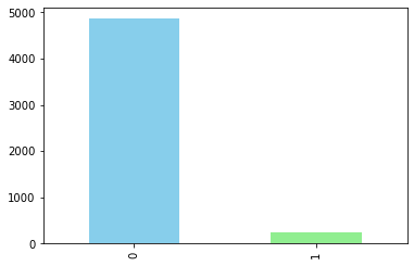
Plot 1: stroke value counts
We’ve an unbalanced dataset with lot’s of samples available for false positive. Has a ratio of 95:5 for True negative: True Positive
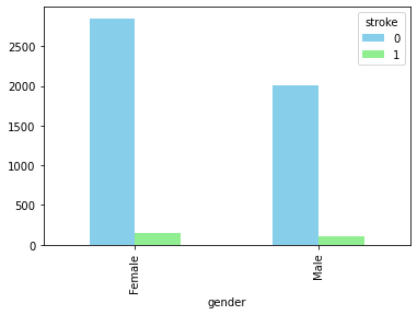
Plot 2: How gender affects stroke
Women are more susceptible to have stroke thanMen, There’s an outlier with one sample in other gender we’ll drop the sample.
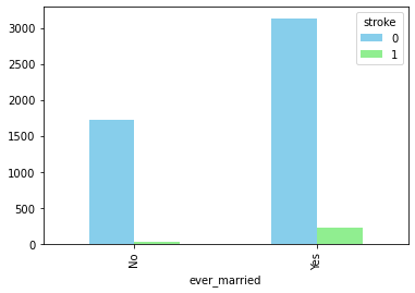
Plot 3: How whether a person is or was married affects stroke
People who is or was married are more susceptible to have stroke. To all the single out there, at least you won’t have stroke any time soon😜🤣.
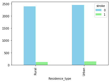
Plot 4: How residence_type impacts stroke
Urban people have a little edge compared to rural people on stroke possiblity.
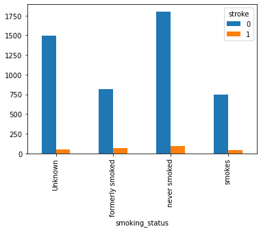
Plot 5: How smoking_type impacts stroke
Smoking is injurious to health and environment. Looking at the plot,smoking has caused a little percent of them a stroke. never smoked are affected by stroke higher than other categories, but never_smoked contributes to 37% of the dataset.
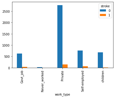
Plot 6: How work_type impacts stroke
People in private are more susceptibe to stroke compared to other categories, but private category contributes to is 57% dataset.
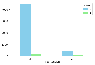
Plot 7: How hyper_tension impacts stroke
Hypertension has high possiblity of becoming a stroke.
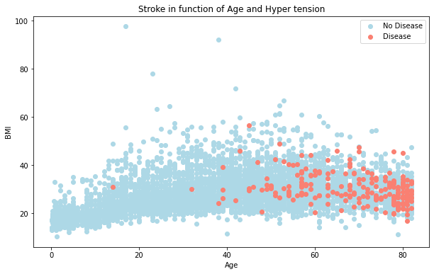
Plot 8: How age, bmi impacts stroke
Older people with low bmi have a possiblity of stroke.
Plot 9: How age, avg_glucose_level impacts stroke
Older people with low glucose level have a possiblity of stroke.
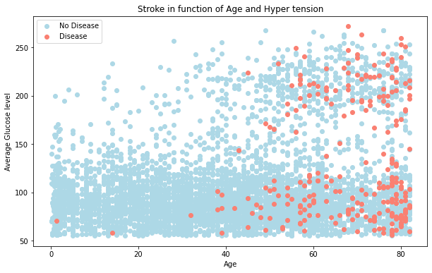
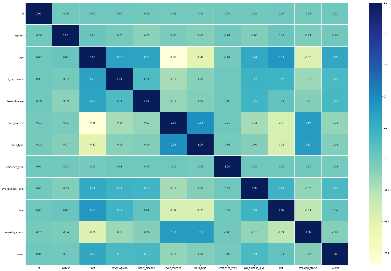
Plot 10: One last EDA for this blog
An correlation matrix between features and how they affect each others.
Preparing the data
The below mentioned categorical features are converted to numerical fetaures.
- gender
- Male: 0
- Female: 1
- ever_married
- Yes: 0
- No: 1
- work_type
- Private: 0
- Self-Employed: 1
- Govt_job: 2
- children: 3
- Never_worked: 4
- Residence_type
- Urban: 0
- Rural: 1
- smoking_status
- formerly smoked: 0
- never smoked: 1
- smoked: 2
- Unknown: 3
Modelling
- The data is splitted into train and test using
train_test_split - Initially We’ve taken the below the classifiers and modelled them on the training data
- KNeighborsClassifier
- LogisticRegression
- RandomForestClassifier
# Put models in a dictionary
models = {"KNN": KNeighborsClassifier(),
          "Logistic Regression": LogisticRegression(),
          "Random Forest": RandomForestClassifier()}

def fit_and_score(models, x_train, x_test, y_train, y_test):
    """
    Model to fit the data to a model and score the model with test data
    models - dictionary of models
    x_train - training features
    x_test - test features
    y_train - training features
    y_test - test_features
    """
    np. random.seed(42)
    model_scores = {}
    for name, model in models.items():
        model.fit(x_train, y_train)
        model_scores[name] = model.score(x_test, y_test)
    return model_scores
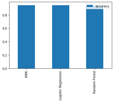
After training we’ve got the below accuracy scores for the models
Hypertuning
Let’s Hypertune the above models to see if we can get better accuracy.
1. KNeighborsClassifier with neigbhors range from (0,21)
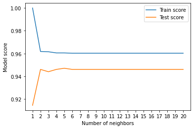
No improvement on model after hypertuning the n_neigbors.
2. RandomizedSearchCV RandomForestClassifier
The below hyperparameters provided better performance than the base model.
{'n_estimators': 260,
 'min_samples_split': 8,
 'min_samples_leaf': 13,
 'max_depth': 10}
Evaluation
Since this is an imbalanced dataset, Accuracy won’t be enough to confirm the model’s performance. There are few ways to work on imbalanced sets.
Let’s find below metrics on how the model performs on both classes - One of the ways to work on imbalanced sets.
1. ROC Curve
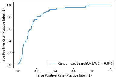
We’ve an AUC of 0.84 which is not bad.
2. Confusion matrix
Confusion matrix will give more clear picture on model’s predictions on majority and minority classes.
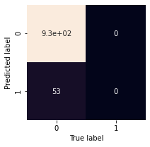
The model is unable to predict anything for class 1. Since machine learning tries to mimize the error at most, model is choosing the majority class which will be at 95%. The minority class is really important for stroke prediction because if we predict True Potive(Stroke) as False Postive(No Stroke) will be major pain to the patients. Let’s see the F1-score and mac-avg as our last evaluation of the model.
3. Classification report
The f1-score for class 1 is 0 and macro avg is 0.49 further confirming classification report, that the model is not at all predicting the minority class.
precision    recall  f1-score   support

           0       0.95      1.00      0.97       929
           1       0.00      0.00      0.00        53

    accuracy                           0.95       982
   macro avg       0.47      0.50      0.49       982
weighted avg       0.89      0.95      0.92       982
Model is not able to predict anything for class 1(0.00), the class imbalance is really big as macrov avg is also really low Okay now we’re getting how big an impact the imbalance dataset is having on our models.
Imbalanced dataset Experimentation
This is my first binary classification modelling experience on an imbalanced dataset. There are two way’s here
- Algorithm-based
- Dataset-based
I went Dataset-based approach. Since am using scikit-learn for modelling, I’ve googled and found imblearn. imblearn has oversampling, undersampling and more methods to play around.
We’ll use the below combination of models and imblearn techniques,
Models
- KNeighborsClassifier
- LogisticRegression
- RandomForest
Samplers
- RandomOverSampler - sampling_strategy=’minority’
- SMOTE - sampling_strategy=’minority’
- ADASYN - sampling_strategy=’minority’
- RandomUnderSampler - sampling_strategy=’majority’
- TomekLinks - sampling_strategy=’majority’
Code snipped for this.
# Put models in a dictionary
models = {"KNN": KNeighborsClassifier(),
          "LogisticRegression": LogisticRegression(),
          "RandomForest": RandomForestClassifier()}

resamplers = {
    "ros": RandomOverSampler(sampling_strategy='minority'),
    "smote": SMOTE(sampling_strategy='minority'),
    "adasyn": ADASYN(sampling_strategy='minority'),
    "rus": RandomUnderSampler(sampling_strategy="majority"),
    "tomek": TomekLinks(sampling_strategy="majority")
}

def fit_resample_and_score(models, samplers, x, y):
    """
    Model to resample data to a model and score the model with test data
    models - dictionary of models
    samplers - samplers to resample the data
    x - features
    y - labels
    """
    np. random.seed(42)
    model_scores = {}
    for sname, sampler in samplers.items():

        # resampling the data
        X_resampled, Y_resampled = sampler.fit_resample(x, y)

        # Splitting the data
        X_train, X_test, Y_train, Y_test = train_test_split(x, y, test_size=0.2)

        for mname, model in models.items():
            #print(sname + mname)
            model.fit(X_train, Y_train)
            model_scores[sname+mname] = model.score(X_test, Y_test)

    return model_scores
Plot comparison visualization of above
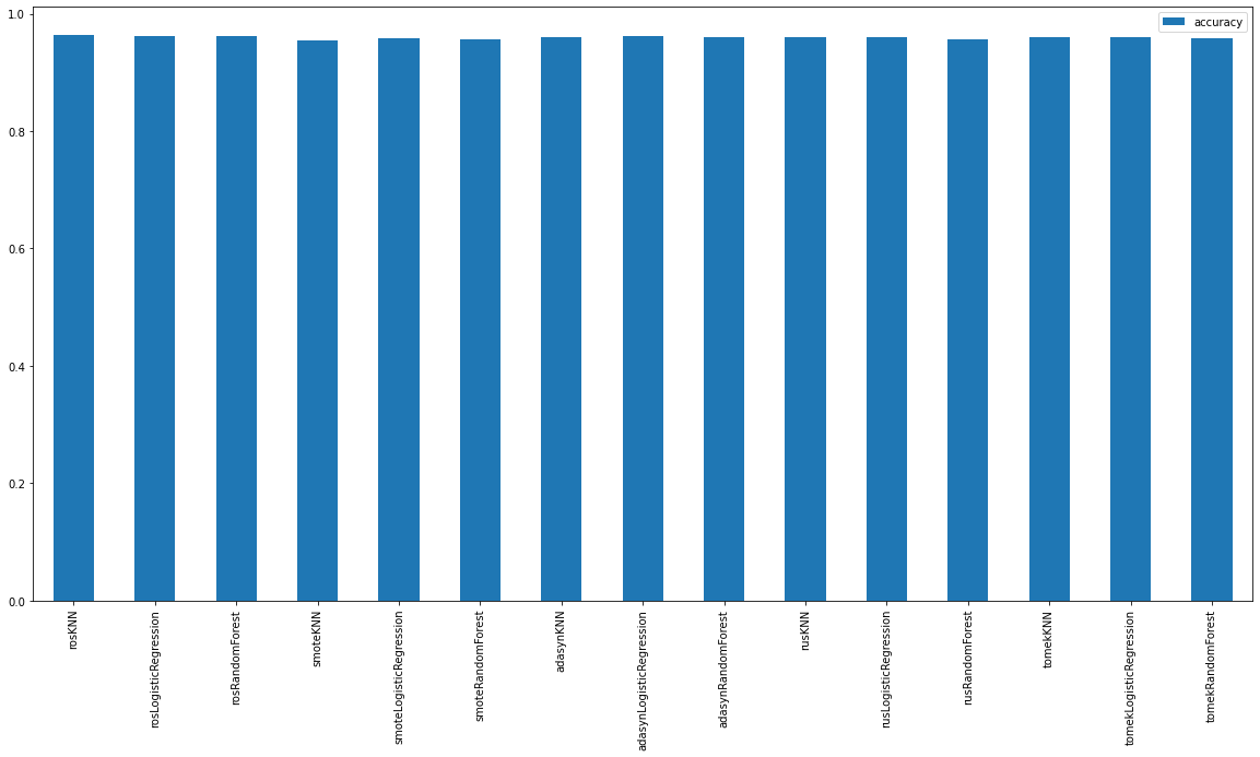
The model with highest accuracy is rosKNN with 0.9633401221995926
Hypertuning
Let’s hypertune the base model with neighbors from range(1,21) to see if we can improve the performace from base model.
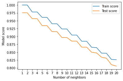
Maximum KNN score on the test data: 97.53% is obtained after hypertuning for n_neighbors=1.
Evaluation metrics
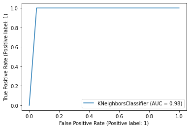
Let’s calculate moed metrics for KNeighborsClassifier with n_neighbors=1.
1. ROC curve
2. ClassificationReport
              precision    recall  f1-score   support

           0       1.00      0.95      0.97      1184
           1       0.95      1.00      0.98      1166

    accuracy                           0.98      2350
   macro avg       0.98      0.98      0.98      2350
weighted avg       0.98      0.98      0.98      2350
We’ve an improved f1-score for both classed and 98%🔥 accuracy which is great😎.
3. ConfusionMatrix
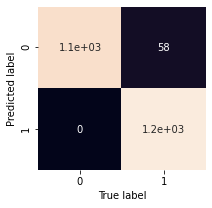
We got only 58 false negatives in resampled dataset.
To conclude I’ve tried to explore how to work on imbalanced dataset in binary classification. Covered few sampling methods from imblearn. Fot this stroke prediction dataset RandomOverSampling KNeighborsClassifier with n_neighbors=1 performs the bset.
Hope you’ve enjoyed the read!!